Model¶

PyEPO supports end-to-end predict-then-optimize with linear objective functions and unknown cost coefficients. At its core is the differentiable optimization solver, which computes gradients of the loss with respect to the cost coefficients.

optModel is the base abstraction in PyEPO. It wraps an optimization solver or algorithm with a unified interface for training and evaluation. PyEPO provides several pre-defined models using GurobiPy, COPT, Pyomo, OR-Tools, and MPAX:

Shortest path (GurobiPy, COPT, Pyomo, OR-Tools & MPAX)
Knapsack (GurobiPy, COPT, Pyomo, OR-Tools & MPAX)
Traveling salesperson (GurobiPy, COPT & Pyomo)
Capacitated vehicle routing (GurobiPy, COPT & Pyomo)
Portfolio optimization (GurobiPy, COPT & Pyomo)

When building models with PyEPO, users do not need to specify the cost coefficients – they are predicted from data at training time.

For more details, see the 01 Optimization Model notebook.

User-Defined Models¶

Users can define custom optimization problems with linear objective functions. PyEPO provides several ways to do this:

GurobiPy-based: Inherit from optGrbModel and implement _getModel.
COPT-based: Inherit from optCoptModel and implement _getModel.
Pyomo-based: Inherit from optOmoModel and implement _getModel.
OR-Tools-based: Inherit from optOrtModel (pywraplp) or optOrtCpModel (CP-SAT) and implement _getModel.
MPAX-based: Inherit from optMpaxModel and implement _getModel to populate constraint matrices self.A, self.b, self.G, self.h, self.l, self.u.
From scratch: Inherit from optModel and implement _getModel, setObj, solve, and num_cost.

The optModel interface consists of:

_getModel: Build and return the optimization model and decision variables.
setObj: Set the objective function with a given cost vector.
solve: Solve the problem and return the optimal solution and objective value.
num_cost: Number of cost coefficients (length of the cost vector).

User-Defined GurobiPy Models¶

To define a GurobiPy model, inherit from pyepo.model.grb.optGrbModel and implement the _getModel method. The model sense (minimize/maximize) is automatically detected from the GurobiPy model.

class pyepo.model.grb.optGrbModel

Abstract base class for GurobiPy-backed optimization models.

Subclasses implement _getModel to build a gurobipy.Model and return (model, variables). The objective sense is auto-detected from the underlying Gurobi model – modelSense does not need to be set manually. Solver output is silenced by default; cost-vector updates use the C-level setAttr("Obj", ...) batch path for efficiency.

Variables:: _model (gurobipy.Model) – underlying Gurobi model

__init__() → None

abstractmethod _getModel() → tuple

An abstract method to build a model from an optimization solver

Returns:: optimization model and variables
Return type:: tuple

property num_cost: int: number of costs to be predicted

relax() → optModel: A method to relax the MIP model. Subclasses should override.

setObj(c: np.ndarray | torch.Tensor | list) → None

A method to set the objective function

Parameters:: c – cost of objective function

solve() → tuple[ndarray, float]

A method to solve the model

Returns:: optimal solution (list) and objective value (float)
Return type:: tuple

For example, consider the following binary optimization problem:

\[\begin{split}\begin{aligned} \max_{x} & \sum_{i=0}^4 c_i x_i \\ s.t. \quad & 3 x_0 + 4 x_1 + 3 x_2 + 6 x_3 + 4 x_4 \leq 12 \\ & 4 x_0 + 5 x_1 + 2 x_2 + 3 x_3 + 5 x_4 \leq 10 \\ & 5 x_0 + 4 x_1 + 6 x_2 + 2 x_3 + 3 x_4 \leq 15 \\ & \forall x_i \in \{0, 1\} \end{aligned}\end{split}\]

Users only need to implement the _getModel method:

import random

import gurobipy as gp
from gurobipy import GRB

from pyepo.model.grb import optGrbModel

class myModel(optGrbModel):

    def _getModel(self):
        # create a model
        m = gp.Model()
        # variables
        x = m.addVars(5, name="x", vtype=GRB.BINARY)
        # model sense
        m.modelSense = GRB.MAXIMIZE
        # constraints
        m.addConstr(3 * x[0] + 4 * x[1] + 3 * x[2] + 6 * x[3] + 4 * x[4] <= 12)
        m.addConstr(4 * x[0] + 5 * x[1] + 2 * x[2] + 3 * x[3] + 5 * x[4] <= 10)
        m.addConstr(5 * x[0] + 4 * x[1] + 6 * x[2] + 2 * x[3] + 3 * x[4] <= 15)
        return m, x

myoptmodel = myModel()
cost = [random.random() for _ in range(myoptmodel.num_cost)] # random cost vector
myoptmodel.setObj(cost) # set objective function
myoptmodel.solve() # solve

User-Defined COPT Models¶

To define a COPT model, inherit from pyepo.model.copt.optCoptModel and implement the _getModel method. The model sense (minimize/maximize) is automatically detected from the COPT model.

class pyepo.model.copt.optCoptModel

Abstract base class for Cardinal Optimizer (COPT) backed models.

Subclasses implement _getModel to build a COPT Model and return (model, variables). The objective sense is auto-detected from the underlying COPT model (no need to set modelSense manually); solver logging is silenced by default. Cost-vector updates use the C-level setInfo("Obj", ...) batch path for efficiency. A process-local COPT Envr singleton is reused across instances to avoid re-booting the license and worker threads on every model build.

Variables:: _model (coptpy.Model) – underlying COPT model

__init__() → None

abstractmethod _getModel() → tuple

An abstract method to build a model from an optimization solver

Returns:: optimization model and variables
Return type:: tuple

property num_cost: int: number of costs to be predicted

setObj(c: np.ndarray | torch.Tensor | list) → None

A method to set the objective function

Parameters:: c – cost of objective function

solve() → tuple[ndarray, float]

A method to solve the model

Returns:: optimal solution and objective value
Return type:: tuple

Here is the same problem implemented with COPT:

import random

from coptpy import Envr, COPT

from pyepo.model.copt import optCoptModel

class myModel(optCoptModel):

    def _getModel(self):
        # create a model
        m = Envr().createModel()
        # variables
        x = m.addVars(range(5), vtype=COPT.BINARY)
        # model sense
        m.setObjSense(COPT.MAXIMIZE)
        # constraints
        m.addConstr(3 * x[0] + 4 * x[1] + 3 * x[2] + 6 * x[3] + 4 * x[4] <= 12)
        m.addConstr(4 * x[0] + 5 * x[1] + 2 * x[2] + 3 * x[3] + 5 * x[4] <= 10)
        m.addConstr(5 * x[0] + 4 * x[1] + 6 * x[2] + 2 * x[3] + 3 * x[4] <= 15)
        return m, x

myoptmodel = myModel()
cost = [random.random() for _ in range(myoptmodel.num_cost)] # random cost vector
myoptmodel.setObj(cost) # set objective function
myoptmodel.solve() # solve

User-Defined Pyomo Models¶

To define a Pyomo model, inherit from pyepo.model.omo.optOmoModel and implement the _getModel method.

class pyepo.model.omo.optOmoModel(solver: str = 'glpk')

Abstract base class for Pyomo-backed optimization models.

Subclasses implement _getModel to build a Pyomo ConcreteModel and return (model, variables). Unlike optGrbModel, the objective sense is not detected automatically – set self.modelSense = EPO.MAXIMIZE in _getModel for maximization problems (default is minimization). The cost vector is wired into the model as a mutable Param so that setObj only updates parameter values rather than rebuilding the objective expression.

Any solver supported by Pyomo can be plugged in via the solver argument (e.g., "glpk", "gurobi", "cbc").

Variables:

_model (pyomo.ConcreteModel) – underlying Pyomo model
solver (str) – name of the Pyomo solver backend

__init__(solver: str = 'glpk') → None

Parameters:: solver – name of the Pyomo solver backend (e.g. "glpk", "gurobi")

abstractmethod _getModel() → tuple

An abstract method to build a model from an optimization solver

Returns:: optimization model and variables
Return type:: tuple

property num_cost: int: number of costs to be predicted

relax() → optModel: A method to relax the MIP model. Subclasses should override.

setObj(c: np.ndarray | torch.Tensor | list) → None

A method to set the objective function

Parameters:: c – cost of objective function

solve() → tuple[ndarray, float]

A method to solve the model

Returns:: optimal solution (np.ndarray) and objective value (float)
Return type:: tuple

Warning

Unlike optGrbModel, optOmoModel requires explicitly setting modelSense in _getModel.

Here is the same problem implemented with Pyomo:

import random

from pyomo import environ as pe

from pyepo.model.omo import optOmoModel
from pyepo import EPO

class myModel(optOmoModel):

    def _getModel(self):
        # sense
        self.modelSense = EPO.MAXIMIZE
        # create a model
        m = pe.ConcreteModel()
        # variables
        x = pe.Var([0,1,2,3,4], domain=pe.Binary)
        m.x = x
        # constraints
        m.cons = pe.ConstraintList()
        m.cons.add(3 * x[0] + 4 * x[1] + 3 * x[2] + 6 * x[3] + 4 * x[4] <= 12)
        m.cons.add(4 * x[0] + 5 * x[1] + 2 * x[2] + 3 * x[3] + 5 * x[4] <= 10)
        m.cons.add(5 * x[0] + 4 * x[1] + 6 * x[2] + 2 * x[3] + 3 * x[4] <= 15)
        return m, x

myoptmodel = myModel(solver="gurobi")
cost = [random.random() for _ in range(myoptmodel.num_cost)] # random cost vector
myoptmodel.setObj(cost) # set objective function
myoptmodel.solve() # solve

User-Defined OR-Tools Models¶

OR-Tools provides two solving paradigms: pywraplp (LP/MIP solvers) and CP-SAT (constraint programming). PyEPO provides base classes for both.

pywraplp – Inherit from pyepo.model.ort.optOrtModel and implement _getModel. The solver parameter selects the backend (e.g., "scip", "glop", "cbc").

class pyepo.model.ort.optOrtModel(solver: str = 'scip')

Abstract base class for OR-Tools pywraplp (LP/MIP) models.

Subclasses implement _getModel to build a pywraplp.Solver and return (model, variables). Unlike optGrbModel, the objective sense is not detected automatically – set self.modelSense = EPO.MAXIMIZE in _getModel for maximization problems (default is minimization). Solver output is silenced by default. The backend solver is selected at construction time via the solver argument (e.g., "scip", "glop", "cbc").

Variables:

_model (pywraplp.Solver) – underlying OR-Tools linear solver
solver (str) – pywraplp backend name

__init__(solver: str = 'scip') → None

Parameters:: solver – pywraplp backend (e.g. "scip", "glop", "cbc")

abstractmethod _getModel() → tuple

An abstract method to build a model from an optimization solver

Returns:: optimization model and variables
Return type:: tuple

property num_cost: int: number of costs to be predicted

setObj(c: np.ndarray | torch.Tensor | list) → None

A method to set the objective function

Parameters:: c – cost of objective function

solve() → tuple[ndarray, float]

A method to solve the model

Returns:: optimal solution (list) and objective value (float)
Return type:: tuple

Warning

Unlike optGrbModel, optOrtModel requires explicitly setting modelSense in _getModel.

import random

from ortools.linear_solver import pywraplp

from pyepo.model.ort import optOrtModel
from pyepo import EPO

class myModel(optOrtModel):

    def _getModel(self):
        # sense
        self.modelSense = EPO.MAXIMIZE
        # create a model
        m = pywraplp.Solver.CreateSolver("SCIP")
        # variables
        x = {i: m.BoolVar(f"x_{i}") for i in range(5)}
        # constraints
        m.Add(3 * x[0] + 4 * x[1] + 3 * x[2] + 6 * x[3] + 4 * x[4] <= 12)
        m.Add(4 * x[0] + 5 * x[1] + 2 * x[2] + 3 * x[3] + 5 * x[4] <= 10)
        m.Add(5 * x[0] + 4 * x[1] + 6 * x[2] + 2 * x[3] + 3 * x[4] <= 15)
        return m, x

myoptmodel = myModel(solver="scip")
cost = [random.random() for _ in range(myoptmodel.num_cost)] # random cost vector
myoptmodel.setObj(cost) # set objective function
myoptmodel.solve() # solve

CP-SAT – Inherit from pyepo.model.ort.optOrtCpModel and implement _getModel. CP-SAT is an integer-only solver; float cost vectors are automatically scaled internally.

class pyepo.model.ort.optOrtCpModel

Abstract base class for OR-Tools CP-SAT (constraint programming) models.

Subclasses implement _getModel to build a cp_model.CpModel and return (model, variables). CP-SAT is an integer-only solver, so float cost vectors are scaled internally (multiplied by _OBJ_SCALE and cast to int) before being passed to the solver; the objective value returned by solve is rescaled back to the original units.

As with the other non-Gurobi/non-COPT backends, modelSense is not auto-detected – set self.modelSense = EPO.MAXIMIZE in _getModel for maximization (default is minimization). CP-SAT does not support LP relaxation, so relax() raises RuntimeError.

Variables:: _model (cp_model.CpModel) – underlying OR-Tools CP-SAT model

__init__() → None

abstractmethod _getModel() → tuple

An abstract method to build a model from an optimization solver

Returns:: optimization model and variables
Return type:: tuple

property num_cost: int: number of costs to be predicted

setObj(c: np.ndarray | torch.Tensor | list) → None

A method to set the objective function

Parameters:: c – cost of objective function

solve() → tuple[ndarray, float]

A method to solve the model

Returns:: optimal solution (list) and objective value (float)
Return type:: tuple

from ortools.sat.python import cp_model

from pyepo.model.ort import optOrtCpModel
from pyepo import EPO

class myCpModel(optOrtCpModel):

    def _getModel(self):
        # sense
        self.modelSense = EPO.MAXIMIZE
        # create a model
        m = cp_model.CpModel()
        # variables
        x = {i: m.NewBoolVar(f"x_{i}") for i in range(5)}
        # constraints (integer coefficients)
        m.Add(3 * x[0] + 4 * x[1] + 3 * x[2] + 6 * x[3] + 4 * x[4] <= 12)
        m.Add(4 * x[0] + 5 * x[1] + 2 * x[2] + 3 * x[3] + 5 * x[4] <= 10)
        m.Add(5 * x[0] + 4 * x[1] + 6 * x[2] + 2 * x[3] + 3 * x[4] <= 15)
        return m, x

myoptmodel = myCpModel()

Note

CP-SAT does not support LP relaxation. Calling relax() will raise a RuntimeError.

User-Defined MPAX Models¶

MPAX (Mathematical Programming in JAX) is a hardware-accelerated mathematical programming framework based on the PDHG (Primal-Dual Hybrid Gradient) algorithm, designed for large-scale linear and quadratic programs.

For a runnable walkthrough that batch-solves LPs on GPU end-to-end with MPAX, see the 09 Solving on MPAX with PDHG notebook.

To define an MPAX model, inherit from pyepo.model.mpax.optMpaxModel and populate the constraint matrices inside _getModel:

self.A, self.b: Equality constraints \(Ax = b\). Use jnp.zeros((0, n)) / jnp.zeros((0,)) for none.

self.G, self.h: Inequality constraints \(Gx \geq h\). Use jnp.zeros((0, n)) / jnp.zeros((0,)) for none.

self.l: Lower bounds (typically zeros for non-negative variables).

self.u: Upper bounds (use jnp.full(n, jnp.inf) for unbounded).

self.Q (optional): PSD quadratic-objective matrix for the QP path; default None keeps the LP path.

_getModel returns (None, []) – MPAX has no explicit model object; the matrices are the model. Additional knobs:

Sparse vs dense: override the class attribute use_sparse_matrix (default True).
Model sense: set self.modelSense = EPO.MAXIMIZE in _getModel or __init__ for a maximization problem; defaults to minimization.
LP vs QP: leave self.Q = None (default) for an LP routed through create_lp; assign a PSD matrix to switch to a convex QP with objective \(\tfrac{1}{2} x^\top Q x + c^\top x\) routed through create_qp. Constraints stay linear – MPAX only supports a quadratic objective. MAXIMIZE with a PSD Q is non-convex and rejected at construction; reformulate as MINIMIZE of the negated objective.

class pyepo.model.mpax.optMpaxModel

Abstract base class for MPAX-backed (JAX) linear / quadratic program models.

MPAX is a JAX implementation of the PDHG (Primal-Dual Hybrid Gradient) first-order solver, designed for large-scale continuous programs that benefit from GPU acceleration and vmap-batched solving. Unlike the Gurobi / COPT / Pyomo / OR-Tools backends, an MPAX model has no explicit solver model object – the constraint matrices and bounds are the model. Subclasses populate them inside _getModel and return (None, []):

def _getModel(self):
    self.A = jnp.array(...)   # equality A x = b
    self.b = jnp.array(...)
    self.G = jnp.array(...)   # inequality G x >= h
    self.h = jnp.array(...)
    self.l = jnp.array(...)   # variable lower bound
    self.u = jnp.array(...)   # variable upper bound
    # optional: leave None for LP, set for convex QP
    self.Q = jnp.array(...)   # PSD; objective is 0.5 xᵀQx + cᵀx
    return None, []

LP vs QP is selected automatically from self.Q: None (default) keeps the LP code path via create_lp, any other value routes through create_qp. Q must be PSD; MPAX supports quadratic objective only – constraints stay linear (this is a hard MPAX limit; e.g. a quadratic risk-budget constraint cannot be expressed).

Objective sense follows self.modelSense (set by a problem-level base such as knapsackBase or directly in _getModel; defaults to minimization). Dense vs sparse matrices can be toggled by overriding the class attribute use_sparse_matrix (default True).

A jitted single-instance solver and a vmap-batched solver (batch_optimize) are pre-compiled on construction, so optDataset can solve every training instance in a single dispatch.

Variables:

A (jnp.ndarray) – equality-constraint matrix (Ax = b)
b (jnp.ndarray) – equality-constraint right-hand side
G (jnp.ndarray) – inequality-constraint matrix (Gx >= h)
h (jnp.ndarray) – inequality-constraint right-hand side
l (jnp.ndarray) – variable lower bounds
u (jnp.ndarray) – variable upper bounds
Q (jnp.ndarray | None) – PSD quadratic-objective matrix; None ⇒ LP
use_sparse_matrix (bool) – whether to use sparse matrices

__init__() → None

abstractmethod _getModel() → tuple

An abstract method to build a model from an optimization solver

Returns:: optimization model and variables
Return type:: tuple

property num_cost: int: number of costs to be predicted

setObj(c: np.ndarray | torch.Tensor | list) → None

A method to set the objective function

Parameters:: c – cost of objective function

solve() → tuple[Tensor, float]

A method to solve the model

Returns:: optimal solution (torch.Tensor) and objective value (float)
Return type:: tuple

import jax.numpy as jnp

from pyepo.model.mpax import optMpaxModel

class myLpModel(optMpaxModel):

    use_sparse_matrix = False  # dense matrices

    def _getModel(self):
        n = 5  # number of variables
        # equality A x = b
        self.A = jnp.array([[1.0, 1.0, 1.0, 1.0, 1.0]])
        self.b = jnp.array([2.0])
        # inequality G x >= h
        self.G = jnp.array([[1.0, 0.0, 1.0, 0.0, 1.0]])
        self.h = jnp.array([1.0])
        # variable bounds x in [0, 1]
        self.l = jnp.zeros(n, dtype=jnp.float32)
        self.u = jnp.ones(n, dtype=jnp.float32)
        return None, []

optmodel = myLpModel()
cost = [0.1, 0.4, 0.2, 0.3, 0.5]
optmodel.setObj(cost) # set objective function
optmodel.solve() # solve

For a QP, additionally assign self.Q to a PSD matrix; the same setObj / solve / batch_optimize interface then minimizes \(\tfrac{1}{2} x^\top Q x + c^\top x\):

import jax.numpy as jnp

from pyepo.model.mpax import optMpaxModel

class myQpModel(optMpaxModel):

    use_sparse_matrix = False

    def _getModel(self):
        n = 4
        # no equality
        self.A = jnp.zeros((0, n), dtype=jnp.float32)
        self.b = jnp.zeros((0,), dtype=jnp.float32)
        # slack inequality so PDHG has a non-empty dual block
        self.G = jnp.ones((1, n), dtype=jnp.float32)
        self.h = jnp.array([-1000.0], dtype=jnp.float32)
        # box bounds
        self.l = jnp.full(n, -10.0, dtype=jnp.float32)
        self.u = jnp.full(n,  10.0, dtype=jnp.float32)
        # PSD quadratic objective -> routes to create_qp
        self.Q = jnp.diag(jnp.array([2.0, 4.0, 6.0, 8.0], dtype=jnp.float32))
        return None, []

optmodel = myQpModel()
optmodel.setObj([-2.0, -4.0, -6.0, -8.0])
optmodel.solve()

User-Defined Models from Scratch¶

For complete flexibility, inherit directly from pyepo.model.opt.optModel to integrate any solver or algorithm. Override _getModel, setObj, solve, and num_cost to provide the same interface as the built-in model wrappers.

class pyepo.model.opt.optModel

Abstract base class for predict-then-optimize models.

Subclasses wrap an optimization solver or algorithm with a unified _getModel / setObj / solve / num_cost interface that pyepo.func modules call during training. Concrete backends are provided for GurobiPy (optGrbModel), Pyomo (optOmoModel), COPT (optCoptModel), OR-Tools (optOrtModel / optOrtCpModel), and MPAX (optMpaxModel); subclass optModel directly to integrate any other solver or algorithm.

The default objective sense is minimization; set self.modelSense = EPO.MAXIMIZE in _getModel or __init__ for maximization problems (some backends, e.g. Gurobi and COPT, detect this automatically from the underlying solver model).

Variables:

_model (optimization model) – underlying solver model object
modelSense (ModelSense) – EPO.MINIMIZE (default) or EPO.MAXIMIZE

__init__() → None

abstractmethod _getModel() → tuple

An abstract method to build a model from an optimization solver

Returns:: optimization model and variables
Return type:: tuple

property num_cost: int: number of costs to be predicted

abstractmethod setObj(c: np.ndarray | torch.Tensor | list) → None

An abstract method to set the objective function

Parameters:: c – cost of objective function

abstractmethod solve() → tuple[np.ndarray | torch.Tensor | list, float]

An abstract method to solve the model

Returns:: optimal solution (list) and objective value (float)
Return type:: tuple

Note

For maximization problems, set self.modelSense = EPO.MAXIMIZE in __init__ or _getModel. Otherwise the default is minimization.

The following example uses networkx with the Dijkstra algorithm to solve a shortest path problem:

import random

import numpy as np
import networkx as nx

from pyepo.model.opt import optModel

class myShortestPathModel(optModel):

    def __init__(self, grid):
        """
        Args:
            grid (tuple): size of grid network
        """
        self.grid = grid
        self.arcs = self._getArcs()
        super().__init__()

    def _getArcs(self):
        """
        A method to get list of arcs for grid network

        Returns:
            list: arcs
        """
        arcs = []
        for i in range(self.grid[0]):
            # edges on rows
            for j in range(self.grid[1] - 1):
                v = i * self.grid[1] + j
                arcs.append((v, v + 1))
            # edges in columns
            if i == self.grid[0] - 1:
                continue
            for j in range(self.grid[1]):
                v = i * self.grid[1] + j
                arcs.append((v, v + self.grid[1]))
        return arcs

    def _getModel(self):
        """
        A method to build model

        Returns:
            tuple: optimization model and variables
        """
        # build graph as optimization model
        g = nx.Graph()
        # add arcs as variables
        g.add_edges_from(self.arcs, cost=0)
        return g, g.edges

    def setObj(self, c):
        """
        A method to set objective function

        Args:
            c (ndarray): cost of objective function
        """
        for i, e in enumerate(self.arcs):
            self._model.edges[e]["cost"] = c[i]

    def solve(self):
        """
        A method to solve model

        Returns:
            tuple: optimal solution (list) and objective value (float)
        """
        # dijkstra
        path = nx.shortest_path(self._model, weight="cost", source=0, target=self.grid[0]*self.grid[1]-1)
        # convert path into active edges
        edges = []
        u = 0
        for v in path[1:]:
            edges.append((u,v))
            u = v
        # init sol & obj
        sol = np.zeros(self.num_cost)
        obj = 0
        # convert active edges into solution and obj
        for i, e in enumerate(self.arcs):
            if e in edges:
                sol[i] = 1 # active edge
                obj += self._model.edges[e]["cost"] # cost of active edge
        return sol, obj

# solve model
grid = (5,5)
myoptmodel = myShortestPathModel(grid)
cost = [random.random() for _ in range(myoptmodel.num_cost)] # random cost vector
myoptmodel.setObj(cost) # set objective function
sol, obj = myoptmodel.solve() # solve
# print res
print('Obj: {}'.format(obj))
for i, e in enumerate(myoptmodel.arcs):
    if sol[i] > 1e-3:
        print(e)

Pre-Defined Models¶

PyEPO includes pre-defined models for several classic optimization problems. Each problem ships with multiple solver backends; the setObj / solve / num_cost interface is identical across them, so you can swap backends without changing the surrounding training code.

Note

In end-to-end training, setObj and solve are invoked automatically inside the pyepo.func modules. The manual setObj / solve calls shown in each example below are for illustration only.

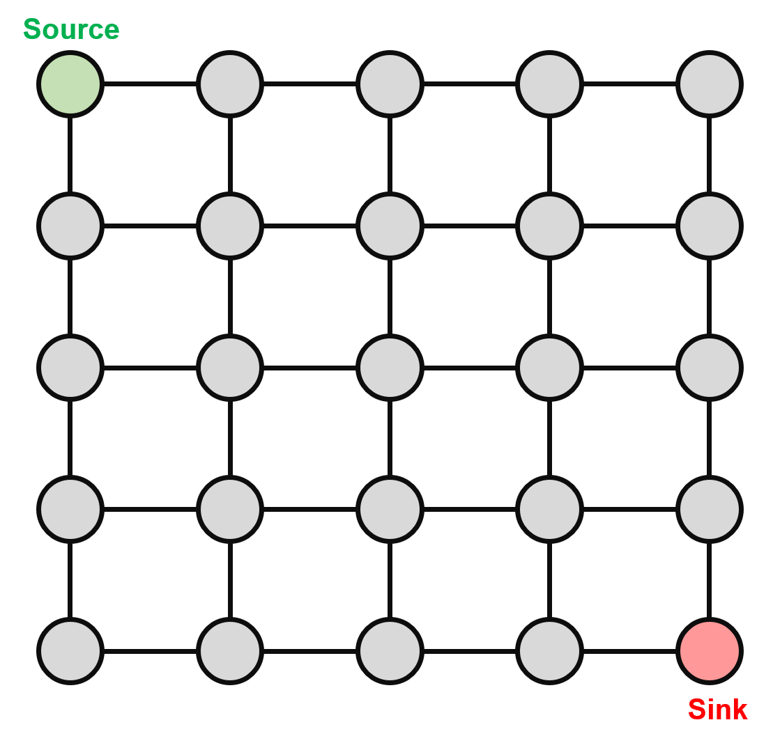
Shortest Path¶

The shortest path problem finds the minimum-cost path from the northwest corner to the southeast corner of an (h, w) grid network. The default grid size is (5, 5). The problem is formulated as a minimum cost flow linear program.

Available backends:

Backend	Class	Notes
GurobiPy	`pyepo.model.grb.shortestPathModel`
COPT	`pyepo.model.copt.shortestPathModel`
Pyomo	`pyepo.model.omo.shortestPathModel`	pick solver via `solver=` (e.g. `"glpk"`, `"gurobi"`)
OR-Tools (pywraplp)	`pyepo.model.ort.shortestPathModel`	pick solver via `solver=` (default `"glop"`, also `"scip"`)
OR-Tools (CP-SAT)	`pyepo.model.ort.shortestPathCpModel`	constraint programming
MPAX	`pyepo.model.mpax.shortestPathModel`	LP on GPU via PDHG

class pyepo.model.grb.shortestPathModel(grid: tuple[int, int], *args, **kwargs)

Gurobi-backed shortest path on a grid network.

Variables:

_model (GurobiPy model) – Gurobi model
grid (tuple of int) – Size of grid network
arcs (list) – List of arcs

__init__(grid: tuple[int, int], *args, **kwargs) → None

Parameters:: grid – grid dimensions (rows, cols)

property num_cost: int: number of costs to be predicted

setObj(c: np.ndarray | torch.Tensor | list) → None

A method to set the objective function

Parameters:: c – cost of objective function

solve() → tuple[ndarray, float]

A method to solve the model

Returns:: optimal solution (list) and objective value (float)
Return type:: tuple

class pyepo.model.copt.shortestPathModel(grid: tuple[int, int], *args, **kwargs)

COPT-backed shortest path on a grid network.

Variables:

_model (COPT model) – COPT model
grid (tuple of int) – Size of grid network
arcs (list) – List of arcs

__init__(grid: tuple[int, int], *args, **kwargs) → None

Parameters:: grid – grid dimensions (rows, cols)

property num_cost: int: number of costs to be predicted

setObj(c: np.ndarray | torch.Tensor | list) → None

A method to set the objective function

Parameters:: c – cost of objective function

solve() → tuple[ndarray, float]

A method to solve the model

Returns:: optimal solution and objective value
Return type:: tuple

class pyepo.model.omo.shortestPathModel(grid: tuple[int, int], solver: str = 'glpk')

Pyomo-backed shortest path on a grid network.

Variables:

_model (Pyomo model) – Pyomo model
solver (str) – optimization solver in the background
grid (tuple of int) – Size of grid network
arcs (list) – List of arcs

__init__(grid: tuple[int, int], solver: str = 'glpk') → None

Parameters:

grid – size of grid network
solver – optimization solver in the background

property num_cost: int: number of costs to be predicted

setObj(c: np.ndarray | torch.Tensor | list) → None

A method to set the objective function

Parameters:: c – cost of objective function

solve() → tuple[ndarray, float]

A method to solve the model

Returns:: optimal solution (np.ndarray) and objective value (float)
Return type:: tuple

class pyepo.model.ort.shortestPathModel(grid: tuple[int, int], solver: str = 'glop')

OR-Tools (pywraplp) backed shortest path on a grid network.

Variables:

_model (pywraplp.Solver) – OR-Tools linear solver
solver (str) – solver backend
grid (tuple of int) – Size of grid network
arcs (list) – List of arcs

__init__(grid: tuple[int, int], solver: str = 'glop') → None

Parameters:

grid – size of grid network
solver – solver backend for pywraplp

property num_cost: int: number of costs to be predicted

setObj(c: np.ndarray | torch.Tensor | list) → None

A method to set the objective function

Parameters:: c – cost of objective function

solve() → tuple[ndarray, float]

A method to solve the model

Returns:: optimal solution (list) and objective value (float)
Return type:: tuple

class pyepo.model.ort.shortestPathCpModel(grid: tuple[int, int], *args, **kwargs)

OR-Tools CP-SAT backed shortest path on a grid network.

Variables:

_model (cp_model.CpModel) – OR-Tools CP-SAT model
grid (tuple of int) – Size of grid network
arcs (list) – List of arcs

__init__(grid: tuple[int, int], *args, **kwargs) → None

Parameters:: grid – grid dimensions (rows, cols)

property num_cost: int: number of costs to be predicted

setObj(c: np.ndarray | torch.Tensor | list) → None

A method to set the objective function

Parameters:: c – cost of objective function

solve() → tuple[ndarray, float]

A method to solve the model

Returns:: optimal solution (list) and objective value (float)
Return type:: tuple

class pyepo.model.mpax.shortestPathModel(grid: tuple[int, int], *args, **kwargs)

MPAX-backed (JAX LP) shortest path on a grid network.

Variables:

grid (tuple of int) – Size of grid network
arcs (list) – List of arcs

__init__(grid: tuple[int, int], *args, **kwargs) → None

Parameters:: grid – grid dimensions (rows, cols)

property num_cost: int: number of costs to be predicted

setObj(c: np.ndarray | torch.Tensor | list) → None

A method to set the objective function

Parameters:: c – cost of objective function

solve() → tuple[Tensor, float]

A method to solve the model

Returns:: optimal solution (torch.Tensor) and objective value (float)
Return type:: tuple

Example:

import pyepo
import random

grid = (5, 5)

# pick a backend (default = GurobiPy)
optmodel = pyepo.model.grb.shortestPathModel(grid)
# alternatives:
# optmodel = pyepo.model.copt.shortestPathModel(grid)
# optmodel = pyepo.model.omo.shortestPathModel(grid, solver="glpk")
# optmodel = pyepo.model.ort.shortestPathModel(grid)            # pywraplp, GLOP default
# optmodel = pyepo.model.ort.shortestPathCpModel(grid)          # CP-SAT
# optmodel = pyepo.model.mpax.shortestPathModel(grid)

cost = [random.random() for _ in range(optmodel.num_cost)]
optmodel.setObj(cost)
sol, obj = optmodel.solve()

Knapsack¶

The multi-dimensional knapsack problem is a maximization problem: select a subset of items such that total weight does not exceed resource capacities and total value is maximized. Consider a 3-dimensional example:

The constraint coefficients weights and right-hand sides capacities define the problem.

Note

The number of dimensions and items are determined by the shape of weights and capacities.

Available backends:

Backend	Class	Notes
GurobiPy	`pyepo.model.grb.knapsackModel`	supports LP relaxation via `relax()`
COPT	`pyepo.model.copt.knapsackModel`	supports `relax()`
Pyomo	`pyepo.model.omo.knapsackModel`	pick solver via `solver=`; supports `relax()`
OR-Tools (pywraplp)	`pyepo.model.ort.knapsackModel`	default solver `"scip"`; supports `relax()`
OR-Tools (CP-SAT)	`pyepo.model.ort.knapsackCpModel`	requires integer coefficients (floats are truncated)
MPAX	`pyepo.model.mpax.knapsackModel`	solves the LP relaxation on GPU via PDHG

class pyepo.model.grb.knapsackModel(weights: ndarray | list, capacity: ndarray | list, *args, **kwargs)

Gurobi-backed knapsack.

Variables:

_model (GurobiPy model) – Gurobi model
weights (np.ndarray) – Weights of items
capacity (np.ndarray) – Total capacity
items (list) – List of item index

__init__(weights: ndarray | list, capacity: ndarray | list, *args, **kwargs) → None

Parameters:

weights – item weights with shape (dim, n_items)
capacity – per-dimension capacity with length dim

property num_cost: int: number of costs to be predicted

relax() → knapsackModelRel: A method to get linear relaxation model

setObj(c: np.ndarray | torch.Tensor | list) → None

A method to set the objective function

Parameters:: c – cost of objective function

solve() → tuple[ndarray, float]

A method to solve the model

Returns:: optimal solution (list) and objective value (float)
Return type:: tuple

class pyepo.model.copt.knapsackModel(weights: ndarray | list, capacity: ndarray | list, *args, **kwargs)

COPT-backed knapsack.

Variables:

_model (COPT model) – COPT model
weights (np.ndarray) – weights of items
capacity (np.ndarray) – total capacity
items (list) – list of item index

__init__(weights: ndarray | list, capacity: ndarray | list, *args, **kwargs) → None

Parameters:

weights – item weights with shape (dim, n_items)
capacity – per-dimension capacity with length dim

property num_cost: int: number of costs to be predicted

relax() → knapsackModelRel: A method to get linear relaxation model

setObj(c: np.ndarray | torch.Tensor | list) → None

A method to set the objective function

Parameters:: c – cost of objective function

solve() → tuple[ndarray, float]

A method to solve the model

Returns:: optimal solution and objective value
Return type:: tuple

class pyepo.model.omo.knapsackModel(weights: ndarray | list, capacity: ndarray | list, solver: str = 'glpk')

Pyomo-backed knapsack.

Variables:

_model (Pyomo model) – Pyomo model
solver (str) – optimization solver in the background
weights (np.ndarray) – weights of items
capacity (np.ndarray) – total capacity
items (list) – list of item index

__init__(weights: ndarray | list, capacity: ndarray | list, solver: str = 'glpk') → None

Parameters:

weights – weights of items
capacity – total capacity
solver – optimization solver in the background

property num_cost: int: number of costs to be predicted

relax() → knapsackModelRel: A method to get linear relaxation model

setObj(c: np.ndarray | torch.Tensor | list) → None

A method to set the objective function

Parameters:: c – cost of objective function

solve() → tuple[ndarray, float]

A method to solve the model

Returns:: optimal solution (np.ndarray) and objective value (float)
Return type:: tuple

class pyepo.model.ort.knapsackModel(weights: ndarray | list, capacity: ndarray | list, *args, **kwargs)

OR-Tools (pywraplp) backed knapsack.

Variables:

_model (pywraplp.Solver) – OR-Tools linear solver
solver (str) – solver backend
weights (np.ndarray) – weights of items
capacity (np.ndarray) – total capacity
items (list) – list of item index

__init__(weights: ndarray | list, capacity: ndarray | list, *args, **kwargs) → None

Parameters:

weights – item weights with shape (dim, n_items)
capacity – per-dimension capacity with length dim

property num_cost: int: number of costs to be predicted

relax() → knapsackModelRel: A method to get linear relaxation model

setObj(c: np.ndarray | torch.Tensor | list) → None

A method to set the objective function

Parameters:: c – cost of objective function

solve() → tuple[ndarray, float]

A method to solve the model

Returns:: optimal solution (list) and objective value (float)
Return type:: tuple

class pyepo.model.ort.knapsackCpModel(weights: ndarray | list, capacity: ndarray | list, *args, **kwargs)

OR-Tools CP-SAT backed knapsack.

Variables:

_model (cp_model.CpModel) – OR-Tools CP-SAT model
weights (np.ndarray) – weights of items
capacity (np.ndarray) – total capacity
items (list) – list of item index

__init__(weights: ndarray | list, capacity: ndarray | list, *args, **kwargs) → None

Parameters:

weights – item weights with shape (dim, n_items)
capacity – per-dimension capacity with length dim

property num_cost: int: number of costs to be predicted

setObj(c: np.ndarray | torch.Tensor | list) → None

A method to set the objective function

Parameters:: c – cost of objective function

solve() → tuple[ndarray, float]

A method to solve the model

Returns:: optimal solution (list) and objective value (float)
Return type:: tuple

class pyepo.model.mpax.knapsackModel(weights: ndarray | list, capacity: ndarray | list, *args, **kwargs)

MPAX-backed (JAX LP) knapsack — LP relaxation.

Variables:

_model – MPAX model
weights (np.ndarray) – Weights of items
capacity (np.ndarray) – Total capacity
items (list) – List of item index

__init__(weights: ndarray | list, capacity: ndarray | list, *args, **kwargs) → None

Parameters:

weights – item weights with shape (dim, n_items)
capacity – per-dimension capacity with length dim

property num_cost: int: number of costs to be predicted

setObj(c: np.ndarray | torch.Tensor | list) → None

A method to set the objective function

Parameters:: c – cost of objective function

solve() → tuple[Tensor, float]

A method to solve the model

Returns:: optimal solution (torch.Tensor) and objective value (float)
Return type:: tuple

Example:

import pyepo
import random

weights = [[3, 4, 3, 6, 4],
           [4, 5, 2, 3, 5],
           [5, 4, 6, 2, 3]]  # constraint coefficients
capacities = [12, 10, 15]    # constraint right-hand sides

# pick a backend (default = GurobiPy)
optmodel = pyepo.model.grb.knapsackModel(weights, capacities)
# alternatives:
# optmodel = pyepo.model.copt.knapsackModel(weights, capacities)
# optmodel = pyepo.model.omo.knapsackModel(weights, capacities, solver="glpk")
# optmodel = pyepo.model.ort.knapsackModel(weights, capacities)         # pywraplp
# optmodel = pyepo.model.ort.knapsackCpModel(weights, capacities)       # CP-SAT
# import numpy as np
# optmodel = pyepo.model.mpax.knapsackModel(np.array(weights), capacities)

cost = [random.random() for _ in range(optmodel.num_cost)]
optmodel.setObj(cost)
sol, obj = optmodel.solve()

# LP relaxation (unavailable for CP-SAT and MPAX backends)
optmodel_rel = optmodel.relax()

Traveling Salesperson¶

The traveling salesperson problem (TSP) seeks the shortest route that visits each city exactly once and returns to the origin. We consider the symmetric TSP with 20 nodes.

Three ILP formulations are available: Dantzig-Fulkerson-Johnson (DFJ), Gavish-Graves (GG), and Miller-Tucker-Zemlin (MTZ).

Available formulations and backends:

Formulation	Backend	Class	Notes
DFJ	GurobiPy	`pyepo.model.grb.tspDFJModel`	lazy subtour-elimination constraints; no `relax()`
DFJ	COPT	`pyepo.model.copt.tspDFJModel`	lazy subtour-elimination constraints; no `relax()`
GG	GurobiPy	`pyepo.model.grb.tspGGModel`	supports `relax()`
GG	COPT	`pyepo.model.copt.tspGGModel`	supports `relax()`
GG	Pyomo	`pyepo.model.omo.tspGGModel`	supports `relax()`
MTZ	GurobiPy	`pyepo.model.grb.tspMTZModel`	supports `relax()`
MTZ	COPT	`pyepo.model.copt.tspMTZModel`	supports `relax()`
MTZ	Pyomo	`pyepo.model.omo.tspMTZModel`	supports `relax()`

Note

DFJ relies on solver callbacks and is therefore unavailable in Pyomo. It also has exponentially many subtour-elimination constraints and does not support LP relaxation.

class pyepo.model.grb.tspDFJModel(num_nodes: int, *args, **kwargs)

Danzig-Fulkerson-Johnson (DFJ) formulation with lazy subtour elimination.

Uses one undirected Var per edge (x[j,i] aliases x[i,j]), so the paired-vars setObj / solve / _addExtraConstr inherited from tspABModel are overridden here.

__init__(num_nodes: int, *args, **kwargs) → None

Parameters:: num_nodes – number of nodes (cities)

property num_cost: int: number of costs to be predicted

setObj(c: np.ndarray | torch.Tensor | list) → None

A method to set the objective function

Parameters:: c – cost vector

solve() → tuple[ndarray, float]: A method to solve model

class pyepo.model.grb.tspGGModel(num_nodes: int, *args, **kwargs)

Gavish-Graves (GG) formulation.

__init__(num_nodes: int, *args, **kwargs) → None

Parameters:: num_nodes – number of nodes (cities)

property num_cost: int: number of costs to be predicted

relax() → tspGGModelRel: A method to get linear relaxation model

setObj(c: np.ndarray | torch.Tensor | list) → None

A method to set the objective function

Parameters:: c – cost vector

solve() → tuple[ndarray, float]: A method to solve model

class pyepo.model.grb.tspMTZModel(num_nodes: int, *args, **kwargs)

Miller-Tucker-Zemlin (MTZ) formulation.

__init__(num_nodes: int, *args, **kwargs) → None

Parameters:: num_nodes – number of nodes (cities)

property num_cost: int: number of costs to be predicted

relax() → tspMTZModelRel: A method to get linear relaxation model

setObj(c: np.ndarray | torch.Tensor | list) → None

A method to set the objective function

Parameters:: c – cost vector

solve() → tuple[ndarray, float]: A method to solve model

class pyepo.model.copt.tspDFJModel(num_nodes: int, *args, **kwargs)

Danzig-Fulkerson-Johnson (DFJ) formulation with lazy subtour elimination.

Uses one undirected Var per edge, so the paired-vars setObj / solve / _addExtraConstr inherited from tspABModel are overridden here.

__init__(num_nodes: int, *args, **kwargs) → None

Parameters:: num_nodes – number of nodes (cities)

property num_cost: int: number of costs to be predicted

setObj(c: np.ndarray | torch.Tensor | list) → None

A method to set the objective function

Parameters:: c – cost vector

solve() → tuple[ndarray, float]: A method to solve model

class pyepo.model.copt.tspGGModel(num_nodes: int, *args, **kwargs)

Gavish-Graves (GG) formulation.

__init__(num_nodes: int, *args, **kwargs) → None

Parameters:: num_nodes – number of nodes (cities)

property num_cost: int: number of costs to be predicted

relax() → tspGGModelRel: A method to get linear relaxation model

setObj(c: np.ndarray | torch.Tensor | list) → None

A method to set the objective function

Parameters:: c – cost vector

solve() → tuple[ndarray, float]: A method to solve model

class pyepo.model.copt.tspMTZModel(num_nodes: int, *args, **kwargs)

Miller-Tucker-Zemlin (MTZ) formulation.

__init__(num_nodes: int, *args, **kwargs) → None

Parameters:: num_nodes – number of nodes (cities)

property num_cost: int: number of costs to be predicted

relax() → tspMTZModelRel: A method to get linear relaxation model

setObj(c: np.ndarray | torch.Tensor | list) → None

A method to set the objective function

Parameters:: c – cost vector

solve() → tuple[ndarray, float]: A method to solve model

class pyepo.model.omo.tspGGModel(num_nodes: int, solver: str = 'glpk')

Gavish-Graves (GG) formulation.

__init__(num_nodes: int, solver: str = 'glpk') → None

Parameters:

num_nodes – number of nodes
solver – optimization solver in the background

property num_cost: int: number of costs to be predicted

relax() → tspGGModelRel: A method to get linear relaxation model

setObj(c: np.ndarray | torch.Tensor | list) → None

A method to set the objective function

Parameters:: c – cost of objective function

solve() → tuple[ndarray, float]: A method to solve model

class pyepo.model.omo.tspMTZModel(num_nodes: int, solver: str = 'glpk')

Miller-Tucker-Zemlin (MTZ) formulation.

__init__(num_nodes: int, solver: str = 'glpk') → None

Parameters:

num_nodes – number of nodes
solver – optimization solver in the background

property num_cost: int: number of costs to be predicted

relax() → tspMTZModelRel: A method to get linear relaxation model

setObj(c: np.ndarray | torch.Tensor | list) → None

A method to set the objective function

Parameters:: c – cost of objective function

solve() → tuple[ndarray, float]: A method to solve model

Example:

import pyepo
import random

num_nodes = 20

# pick a formulation × backend (default = GurobiPy DFJ)
optmodel = pyepo.model.grb.tspDFJModel(num_nodes)
# alternatives:
# optmodel = pyepo.model.grb.tspGGModel(num_nodes)
# optmodel = pyepo.model.grb.tspMTZModel(num_nodes)
# optmodel = pyepo.model.copt.tspDFJModel(num_nodes)
# optmodel = pyepo.model.copt.tspGGModel(num_nodes)
# optmodel = pyepo.model.copt.tspMTZModel(num_nodes)
# optmodel = pyepo.model.omo.tspGGModel(num_nodes, solver="gurobi")
# optmodel = pyepo.model.omo.tspMTZModel(num_nodes, solver="glpk")

cost = [random.random() for _ in range(optmodel.num_cost)]
optmodel.setObj(cost)
sol, obj = optmodel.solve()

Capacitated Vehicle Routing¶

The capacitated vehicle routing problem (CVRP) seeks the shortest set of vehicle routes that serves every customer exactly once and respects per-vehicle capacity. Each route starts and ends at the depot (node 0), and the depot has degree \(2 k\) where \(k\) is the number of routes used.

Two ILP formulations are available:

Rounded Capacity Inequalities (RCI): undirected 2-degree formulation with lazy rounded-capacity cuts. Requires solver callbacks.
Miller-Tucker-Zemlin (MTZ): directed formulation with per-node load auxiliaries; no callbacks required.

Note

Single-customer routes are excluded so that all edge variables stay strictly binary. If a single-stop route is genuinely required, duplicate the depot node.

Available formulations and backends:

Formulation	Backend	Class	Notes
RCI	GurobiPy	`pyepo.model.grb.vrpRCIModel`	lazy rounded-capacity cuts
RCI	COPT	`pyepo.model.copt.vrpRCIModel`	lazy rounded-capacity cuts
MTZ	GurobiPy	`pyepo.model.grb.vrpMTZModel`	supports `relax()`
MTZ	COPT	`pyepo.model.copt.vrpMTZModel`	supports `relax()`
MTZ	Pyomo	`pyepo.model.omo.vrpMTZModel`	supports `relax()`

Note

Pyomo lacks a native callback API, so only the MTZ formulation is provided.

class pyepo.model.grb.vrpRCIModel(num_nodes: int, demands: list[float] | ndarray, capacity: float, num_vehicle: int)

CVRP formulation with 2-degree constraints and lazy rounded-capacity cuts.

Uses one undirected Var per edge (x[j,i] aliases x[i,j]). Subtour elimination and rounded capacity inequalities are added lazily during branch-and-cut; the cuts added at the optimum are tracked on model._lazy_constrs for downstream CaVE cone extraction.

__init__(num_nodes: int, demands: list[float] | ndarray, capacity: float, num_vehicle: int) → None

Parameters:

num_nodes – number of nodes (depot is node 0)
demands – per-customer demands, length num_nodes - 1
capacity – vehicle capacity
num_vehicle – number of vehicles

getTour(sol: np.ndarray | torch.Tensor | list) → list[list[int]]

Reconstruct vehicle tours from an undirected edge-selection vector.

Parameters:: sol – per-edge selection values aligned with self.edges
Returns:: list of tours; each tour is a node sequence starting and ending at the depot

property num_cost: int: number of costs to be predicted

setObj(c: np.ndarray | torch.Tensor | list) → None

A method to set the objective function

Parameters:: c – cost vector aligned with self.edges

solve() → tuple[ndarray, float]

A method to solve the model

Returns:: edge-selection vector (uint8) and objective value (float)
Return type:: tuple

class pyepo.model.grb.vrpMTZModel(num_nodes: int, demands: list[float] | ndarray, capacity: float, num_vehicle: int)

CVRP formulation on a directed graph with MTZ-style capacity constraints (no lazy cuts). Cost vector is per undirected edge: cost c[k] is assigned to both x[i,j] and x[j,i].

__init__(num_nodes: int, demands: list[float] | ndarray, capacity: float, num_vehicle: int) → None

Parameters:

num_nodes – number of nodes (depot is node 0)
demands – per-customer demands, length num_nodes - 1
capacity – vehicle capacity
num_vehicle – number of vehicles

getTour(sol: np.ndarray | torch.Tensor | list) → list[list[int]]

Reconstruct vehicle tours from an undirected edge-selection vector.

Parameters:: sol – per-edge selection values aligned with self.edges
Returns:: list of tours; each tour is a node sequence starting and ending at the depot

property num_cost: int: number of costs to be predicted

relax() → vrpMTZModelRel: A method to get linear relaxation model

setObj(c: np.ndarray | torch.Tensor | list) → None

A method to set the objective function

Parameters:: c – cost vector aligned with self.edges (one cost per undirected edge)

solve() → tuple[ndarray, float]

A method to solve the model

Returns:: edge-selection vector (uint8) and objective value (float)
Return type:: tuple

class pyepo.model.copt.vrpRCIModel(num_nodes: int, demands: list[float] | ndarray, capacity: float, num_vehicle: int)

CVRP formulation with 2-degree constraints and lazy rounded-capacity cuts.

Uses one undirected Var per edge (x[j,i] aliases x[i,j]). Subtour elimination and rounded capacity inequalities are added lazily during branch-and-cut via a COPT callback.

__init__(num_nodes: int, demands: list[float] | ndarray, capacity: float, num_vehicle: int) → None

Parameters:

num_nodes – number of nodes (depot is node 0)
demands – per-customer demands, length num_nodes - 1
capacity – vehicle capacity
num_vehicle – number of vehicles

getTour(sol: np.ndarray | torch.Tensor | list) → list[list[int]]

Reconstruct vehicle tours from an undirected edge-selection vector.

Parameters:: sol – per-edge selection values aligned with self.edges
Returns:: list of tours; each tour is a node sequence starting and ending at the depot

property num_cost: int: number of costs to be predicted

setObj(c: np.ndarray | torch.Tensor | list) → None

A method to set the objective function

Parameters:: c – cost vector aligned with self.edges

solve() → tuple[ndarray, float]

A method to solve the model

Returns:: edge-selection vector (uint8) and objective value (float)
Return type:: tuple

class pyepo.model.copt.vrpMTZModel(num_nodes: int, demands: list[float] | ndarray, capacity: float, num_vehicle: int)

CVRP formulation on a directed graph with MTZ-style capacity constraints (no lazy cuts). Cost vector is per undirected edge: cost c[k] is assigned to both x[i,j] and x[j,i].

__init__(num_nodes: int, demands: list[float] | ndarray, capacity: float, num_vehicle: int) → None

Parameters:

num_nodes – number of nodes (depot is node 0)
demands – per-customer demands, length num_nodes - 1
capacity – vehicle capacity
num_vehicle – number of vehicles

getTour(sol: np.ndarray | torch.Tensor | list) → list[list[int]]

Reconstruct vehicle tours from an undirected edge-selection vector.

Parameters:: sol – per-edge selection values aligned with self.edges
Returns:: list of tours; each tour is a node sequence starting and ending at the depot

property num_cost: int: number of costs to be predicted

relax() → vrpMTZModelRel: A method to get linear relaxation model

setObj(c: np.ndarray | torch.Tensor | list) → None

A method to set the objective function

Parameters:: c – cost vector aligned with self.edges (one cost per undirected edge)

solve() → tuple[ndarray, float]

A method to solve the model

Returns:: edge-selection vector (uint8) and objective value (float)
Return type:: tuple

class pyepo.model.omo.vrpMTZModel(num_nodes: int, demands: list[float] | ndarray, capacity: float, num_vehicle: int, solver: str = 'glpk')

CVRP formulation on a directed graph with MTZ-style capacity constraints. Cost vector is per undirected edge: cost c[k] is assigned to both x[i,j] and x[j,i].

__init__(num_nodes: int, demands: list[float] | ndarray, capacity: float, num_vehicle: int, solver: str = 'glpk') → None

Parameters:

num_nodes – number of nodes (depot is node 0)
demands – per-customer demands, length num_nodes - 1
capacity – vehicle capacity
num_vehicle – number of vehicles
solver – optimization solver in the background

getTour(sol: np.ndarray | torch.Tensor | list) → list[list[int]]

Reconstruct vehicle tours from an undirected edge-selection vector.

Parameters:: sol – per-edge selection values aligned with self.edges
Returns:: list of tours; each tour is a node sequence starting and ending at the depot

property num_cost: int: number of costs to be predicted

relax() → vrpMTZModelRel: A method to get linear relaxation model

setObj(c: np.ndarray | torch.Tensor | list) → None

A method to set the objective function

Parameters:: c – cost of objective function

solve() → tuple[ndarray, float]

A method to solve the model

Returns:: edge-selection vector (uint8) and objective value (float)
Return type:: tuple

Example:

import pyepo

num_nodes = 10                       # depot + 9 customers
demands = [2, 1, 3, 2, 1, 2, 1, 3, 2]
capacity = 5.0
num_vehicle = 3

# pick a formulation × backend (default = GurobiPy RCI)
optmodel = pyepo.model.grb.vrpRCIModel(num_nodes, demands, capacity, num_vehicle)
# alternatives:
# optmodel = pyepo.model.grb.vrpMTZModel(num_nodes, demands, capacity, num_vehicle)
# optmodel = pyepo.model.copt.vrpRCIModel(num_nodes, demands, capacity, num_vehicle)
# optmodel = pyepo.model.copt.vrpMTZModel(num_nodes, demands, capacity, num_vehicle)
# optmodel = pyepo.model.omo.vrpMTZModel(num_nodes, demands, capacity, num_vehicle)

Portfolio¶

Portfolio optimization selects an asset allocation that maximizes expected return for a given level of risk:

\[\begin{split}\begin{aligned} \max_{x} & \sum_{i} r_i x_i \\ s.t. \quad & \sum_{i} x_i = 1 \\ & \mathbf{x}^{\intercal} \mathbf{\Sigma} \mathbf{x} \leq \gamma \bar{\Sigma}\\ & \forall x_i \geq 0 \end{aligned}\end{split}\]

Available backends:

Backend	Class	Notes
GurobiPy	`pyepo.model.grb.portfolioModel`
COPT	`pyepo.model.copt.portfolioModel`
Pyomo	`pyepo.model.omo.portfolioModel`	pick solver via `solver=`

class pyepo.model.grb.portfolioModel(num_assets: int, covariance: ndarray, gamma: float = 2.25, *args, **kwargs)

Gurobi-backed Markowitz portfolio.

Variables:

_model (GurobiPy model) – Gurobi model
num_assets (int) – number of assets
covariance (numpy.ndarray) – covariance matrix of the returns
risk_level (float) – risk level

__init__(num_assets: int, covariance: ndarray, gamma: float = 2.25, *args, **kwargs) → None

Parameters:

num_assets – number of assets
covariance – covariance matrix of the asset returns
gamma – risk tolerance multiplier on the mean covariance

property num_cost: int: number of costs to be predicted

setObj(c: np.ndarray | torch.Tensor | list) → None

A method to set the objective function

Parameters:: c – cost of objective function

solve() → tuple[ndarray, float]

A method to solve the model

Returns:: optimal solution (list) and objective value (float)
Return type:: tuple

class pyepo.model.copt.portfolioModel(num_assets: int, covariance: ndarray, gamma: float = 2.25, *args, **kwargs)

COPT-backed Markowitz portfolio.

Variables:

_model (COPT model) – COPT model
num_assets (int) – number of assets
covariance (numpy.ndarray) – covariance matrix of the returns
risk_level (float) – risk level

__init__(num_assets: int, covariance: ndarray, gamma: float = 2.25, *args, **kwargs) → None

Parameters:

num_assets – number of assets
covariance – covariance matrix of the asset returns
gamma – risk tolerance multiplier on the mean covariance

property num_cost: int: number of costs to be predicted

setObj(c: np.ndarray | torch.Tensor | list) → None

A method to set the objective function

Parameters:: c – cost of objective function

solve() → tuple[ndarray, float]

A method to solve the model

Returns:: optimal solution and objective value
Return type:: tuple

class pyepo.model.omo.portfolioModel(num_assets: int, covariance: np.ndarray, gamma: float = 2.25, solver: str = 'glpk')

Pyomo-backed Markowitz portfolio.

Variables:

_model (Pyomo model) – Pyomo model
solver (str) – optimization solver in the background
num_assets (int) – number of assets
covariance (numpy.ndarray) – covariance matrix of the returns
risk_level (float) – risk level

__init__(num_assets: int, covariance: np.ndarray, gamma: float = 2.25, solver: str = 'glpk') → None

Parameters:

num_assets – number of assets
covariance – covariance matrix of the returns
gamma – risk level parameter
solver – optimization solver in the background

property num_cost: int: number of costs to be predicted

setObj(c: np.ndarray | torch.Tensor | list) → None

A method to set the objective function

Parameters:: c – cost of objective function

solve() → tuple[ndarray, float]

A method to solve the model

Returns:: optimal solution (np.ndarray) and objective value (float)
Return type:: tuple

Example:

import pyepo
import numpy as np
import random

m = 50  # number of assets
cov = np.cov(np.random.randn(10, m), rowvar=False)

# pick a backend (default = GurobiPy)
optmodel = pyepo.model.grb.portfolioModel(m, cov)
# alternatives:
# optmodel = pyepo.model.copt.portfolioModel(m, cov)
# optmodel = pyepo.model.omo.portfolioModel(m, cov, solver="gurobi")

revenue = [random.random() for _ in range(optmodel.num_cost)]
optmodel.setObj(revenue)
sol, obj = optmodel.solve()