Cone-Aligned Estimation

Cone-aligned losses supervise the predicted cost vector directly. They align it with the polyhedral cone of binding-constraint normals at the true optimum, rather than supervising the optimal solution itself.

The training loop on this page builds on the Common Setup from Training Methods.

Cone-Aligned Vector Estimation (CaVE)

CaVE [1] is a surrogate loss for binary linear programs such as TSP, CVRP, knapsack, and shortest path with binary edges. For each instance, it projects the sense-flipped predicted cost vector onto the polyhedral cone spanned by the binding-constraint normals at the true optimal vertex, then minimizes 1 - cos(pred, proj).

For a runnable walkthrough, see the 04 CaVE for Binary Linear Programs notebook.

Let \(K(\mathbf{w}^*(\mathbf{c}))\) be the polyhedral cone spanned by the constraint normals that bind at the true optimal vertex. For a minimization problem, the KKT conditions require \(-\hat{\mathbf{c}} \in K(\mathbf{w}^*(\mathbf{c}))\) for \(\mathbf{w}^*(\mathbf{c})\) to remain optimal under the predicted cost. CaVE measures this alignment via a cosine loss against the cone projection \(\mathbf{p} = \mathrm{proj}_{K}(-\hat{\mathbf{c}})\),

\[\mathcal{L}_{\mathrm{CaVE}}(\hat{\mathbf{c}}, K) = 1 - \frac{(-\hat{\mathbf{c}})^\top \mathbf{p}}{\|\hat{\mathbf{c}}\|_2\, \|\mathbf{p}\|_2}.\]

When \(-\hat{\mathbf{c}}\) already lies inside the cone, \(\mathbf{p} = -\hat{\mathbf{c}}\) and the loss is zero. The further \(-\hat{\mathbf{c}}\) strays outside the cone, the larger the loss.

CaVE uses two solvers at different stages. A Gurobi-backed optModel extracts the binding-constraint normals when the dataset is built, and Clarabel projects the predicted cost onto that cone during training. This avoids solving an ILP in every training step. max_iter caps the Clarabel iterations. The default max_iter=3 is the paper’s CaVE+ preset, which under-converges the projection on purpose so it stays inside the cone. Raising it changes the loss, not just its precision.

Setting solve_ratio < 1 enables the CaVE-Hybrid update: each batch uses the QP projection with probability solve_ratio and otherwise uses a blend of the normalized predicted cost and the average binding-constraint normal. inner_ratio controls the blend.

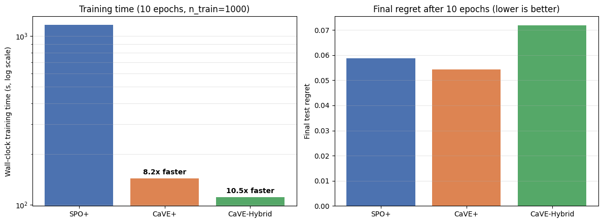
CVRP-20 results from notebook 04: num_data=1000, 10 epochs, single process. In this setup, CaVE+ trains 8.2x faster than SPO+. CaVE-Hybrid with solve_ratio=0.3 trains 10.5x faster than SPO+, with a final regret higher than both.

Training data comes from pyepo.data.dataset.optDatasetConstrs, which extracts the binding-constraint normals at the optimum for each instance. Per-instance constraint counts are ragged, so batch the dataset with pyepo.data.dataset.optDataLoader. It zero-pads the constraint matrices automatically. CaVE currently requires a Gurobi-backed optModel.

pyepo.func.CaVE

alias of coneAlignedCosine

Training loop (the batch carries tight_ctrs in addition to (x, c, w, z)):

from pyepo.data.dataset import optDatasetConstrs, optDataLoader

dataset_constr = optDatasetConstrs(optmodel, feat, costs)
dataloader_constr = optDataLoader(dataset_constr, batch_size=32, shuffle=True)

cave = pyepo.func.CaVE(optmodel, processes=1)

for epoch in range(20):
    for x, c, w, z, tight_ctrs in dataloader_constr:
        cp = predmodel(x)
        loss = cave(cp, tight_ctrs)
        optimizer.zero_grad()
        loss.backward()
        optimizer.step()

If you use the CaVE loss, please cite:

@inproceedings{tang2024cave,
  title={CaVE: A Cone-Aligned Approach for Fast Predict-then-Optimize with Binary Linear Programs},
  author={Tang, Bo and Khalil, Elias B},
  booktitle={Integration of Constraint Programming, Artificial Intelligence, and Operations Research},
  pages={193--210},
  year={2024},
  publisher={Springer}
}

Footnotes

[1]

Tang, B., & Khalil, E. B. (2024). CaVE: A Cone-Aligned Approach for Fast Predict-then-Optimize with Binary Linear Programs. In Integration of Constraint Programming, Artificial Intelligence, and Operations Research (pp. 193-210).