Training Methods

Overview

pyepo.func provides PyTorch autograd modules that wrap an optimization solver for end-to-end training. All modules assume a linear objective with known, fixed constraints. The cost vector is predicted from contextual features. If a DSL-compiled model includes a quadratic objective term, the training module raises at construction.

Every module accepts processes for parallel solving. All modules except CaVE accept solve_ratio < 1 with dataset for solution-pool caching (see Solution Pool). CaVE uses solve_ratio for its projection branch instead. Modules that return a loss also accept reduction ("mean", "sum", or "none").

Each method family has its own page, linked under Method Families below. Every training loop there is presented with its definition and builds on the shared Common Setup on this page.

Choosing a Method

The modules differ in what they return, which determines how you use them:

• Loss-returning: return a scalar loss that can be passed directly to .backward(): SPO+, PG, PFYL, RFYL, CaVE, NCE, CMAP, LTR.

• Solution-returning: return a predicted, expected, or regularized solution. You then define a task loss on that output: DPO, I-MLE, AI-MLE, RFWO, DBB, NID.

A combined name like DPO+MSE or NID+L1 denotes a solution-returning module (DPO, NID) followed by a task loss (here MSE or L1) on its output.

The table below summarizes each module’s return type, typical supervision signal, and main caveats.

Module	Returns	Typical supervision	Notes
SPOPlus	loss	true costs, true optimal solutions, true objective values	convex surrogate for regret
PG	loss	true costs	directional finite differences along the true cost
DPO / DPOMul	expected perturbed solutions	task loss chosen by the user	use the multiplicative variant for sign-sensitive oracles
PFY / PFYMul	loss	true optimal solutions	PFYL; use the multiplicative variant for sign-sensitive oracles
IMLE / AIMLE	expected perturbed solutions	task loss chosen by the user	perturb-and-MAP with Sum-of-Gamma noise
RFWO	regularized predicted solutions	task loss chosen by the user	L2-regularized smooth optimizer over the convex hull of feasible solutions
RFY	loss	true optimal solutions	RFYL; Fenchel-Young loss paired with L2-regularized Frank-Wolfe
DBB / NID	predicted solutions	task loss chosen by the user	direct solution-level or objective-level losses
CaVE	loss	tight binding-constraint normals at the true optimum (optDatasetConstrs)	binary linear programs, Gurobi backend only
NCE / CMAP	loss	true optimal solutions and a solution pool	contrastive training with cached negative solutions
ptLTR / prLTR / lsLTR	loss	true costs and a solution pool	learning-to-rank formulations over feasible solutions

Method Families

Each family has its own page:

• Surrogate Losses
• Perturbed Methods
• Regularized Methods
• Black-Box Methods
• Cone-Aligned Estimation
• Contrastive Methods
• Learning to Rank

Common Setup

All training loops share the same setup: a DSL-defined knapsack problem with a linear predictor. The examples use PyTorch. JAX follows the same method families. See JAX Frontend. For a runnable walkthrough, see the 03 Training and Testing notebook.

import pyepo
from pyepo import EPO, dsl
import torch
from torch import nn
from torch.utils.data import DataLoader

# generate data
num_data, num_feat, num_item, num_dim = 1000, 5, 10, 3
weights, feat, costs = pyepo.data.knapsack.genData(
    num_data, num_feat, num_item, num_dim, deg=4, noise_width=0.5, seed=135,
)
capacity = (weights.sum(axis=1) * 0.5).astype(int)

# define the optimization problem
x = dsl.Variable(num_item, vtype=EPO.BINARY)
c = dsl.Parameter(num_item)
optmodel = dsl.Problem(
    dsl.Maximize(c @ x),
    [weights @ x <= capacity],
).compile(backend="gurobi")

# dataset and data loader
dataset = pyepo.data.dataset.optDataset(optmodel, feat, costs)
dataloader = DataLoader(dataset, batch_size=32, shuffle=True)

# prediction model
predmodel = nn.Linear(num_feat, num_item)
optimizer = torch.optim.Adam(predmodel.parameters(), lr=1e-3)

# for multiplicative perturbed variants
positive_predmodel = nn.Sequential(nn.Linear(num_feat, num_item), nn.Softplus())

Parallel Computation

All pyepo.func modules support parallel solving during training through the processes parameter. Set processes=0 to use all available cores.

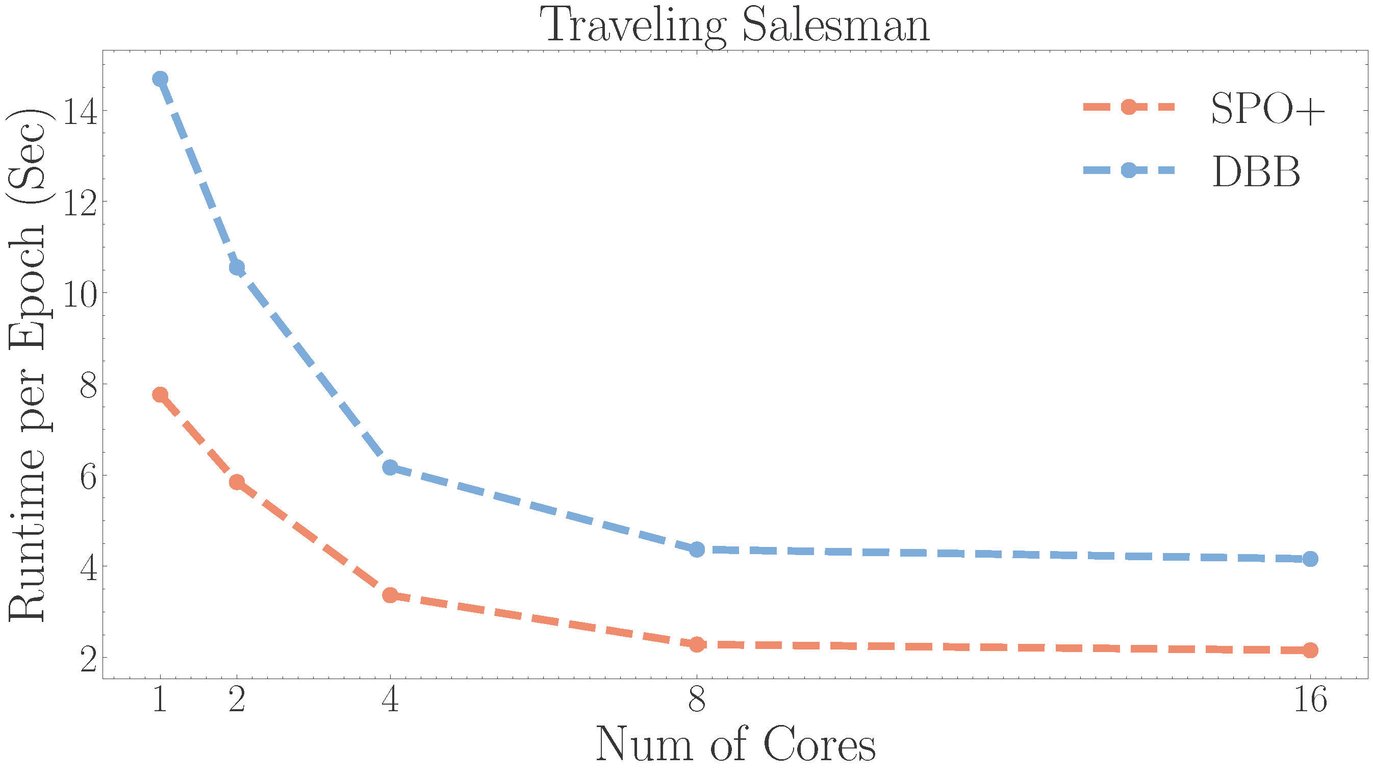
The figure reports runtime for different values of processes.